使用模型
模型转换
The SyNAP toolkit allows to convert a model from its original format to
an internal representation optimized for the target hardware.
The conversion tool and utilities can run on Linux, MacOS or Windows hosts inside a Docker container.
Only Docker and the toolkit image are required, no additional dependencies have to be installed.
The following network model formats are supported:
Tensorflow Lite (
.tfliteextension)ONNX (
.onnxextension)TorchScript (
.torchscript,.pt,.pthextensions)Tensorflow (
.pbextension)Caffe (
.prototxtextension)
备注
PyTorch models can be saved in different formats, only TorchScript format is supported. see 使用 PyTorch 模型 for more information.
备注
Only standard Caffe 1.0 models are supported. Custom variants such as Caffe-SSD or Caffe-LSTM models or legacy (pre-1.0) models require specific parsers which are currently not available in SyNAP toolkit. Caffe2 models are not supported as well.
警告
The support for .pb and .prototxt formats will be removed in the future.
安装Docker
A few installation hints here below, please note that these are not a replacement for the official Docker documentation, for more details please refer to https://docs.docker.com/get-docker/.
Linux/Ubuntu
apt-get install docker.io
To be able to run docker without super user also run the two commands here below once after docker installation (for more info refer to https://docs.docker.com/engine/install/linux-postinstall/).
# Create the docker group if it doesn't already exist
sudo groupadd docker
# Add the current user "$USER" to the docker group
sudo usermod -aG docker $USER
macOS - Docker
The easiest way to install Docker on MacOS is via the brew package manager. If you don't have it installed yet please follow the official brew website: https://brew.sh/ After brew is installed you can install Docker.
重要
On macOS the Docker GUI is not free for use for commercial application, a valid alternative is Colima.
brew install docker
See the note in the linux installation above to run docker without super user.
macOS - Colima
Colima is a free container runtimes on macOS that can be used a replacement for Docker.( https://github.com/abiosoft/colima ). It doesn't have a GUI but nevertheless is easy to install and configure.
brew install colima
mkdir -p ~/.docker/cli-plugins
brew install docker-Buildx
ln -sfn $(brew --prefix)/opt/docker-buildx/bin/docker-buildx ~/.docker/cli-plugins/docker-buildx
colima start --vm-type vz --mount-type virtiofs --cpu 4 --memory 8 --disk 80
After the above commands, you can use Colima to work with Docker containers, the settings are
stored in a config file ~/.colima/default/colima.yaml and can be modified by editing the file
if needed.
Colima has to be started after each restart of the Mac:
colima start
Windows
The suggested way to run Docker on Windows is to install it inside a Linux Virtual Machine using WSL2 available from Windows 10.
重要
Running Docker directly in Windows is incompatible with the presence of a VM. For this reason using a Linux VM in WSL2 is usually the best option.
WSL2 installation steps:
Run Windows PowerShell App as Administrator and execute the following command to install WSL2:
> wsl --installWhen completed restart the computer.
Run Windows PowerShell App as before and install Ubuntu-22.04:
> wsl --install -d Ubuntu-22.04Run Windows Terminal App and select the Ubuntu-22.04 distribution. From there install Docker and the SyNAP toolkit following the instructions in Linux/Ubuntu above
For more information on WSL2 installation and setup please refer to the official Microsoft documentation: https://learn.microsoft.com/en-us/windows/wsl/install and https://learn.microsoft.com/en-us/windows/wsl/setup/environment .
安装 SyNAP 工具
Before installing the SyNAP toolkit, please be sure that you have a working Docker installation.
The simplest way to do this is to run the hello-world image:
$ docker run hello-world

Unable to find image 'hello-world:latest' locally
latest: Pulling from library/hello-world
...
...
...
Hello from Docker!
This message shows that your installation appears to be working correctly.
...
...
If the above command doesn’t produce the expected output please check the instructions in the previous section or refer to the official Docker documentation for your platform. If all is well you can proceed with the installation of the toolkit.
The SyNAP toolkit is distributed as a Docker image, to install it just download the image from the SyNAP github repository:
docker pull ghcr.io/synaptics-synap/toolkit:#SyNAP_Version#
This image contains not only the conversion tool itself but also all the required dependencies and additional support utilities.
You can find the latest version of the toolkit in: SyNAP 下载
运行 SyNAP 工具
Once Docker and the SyNAP toolkit image are installed, the model conversion tool can be executed
directly inside a docker container.
The source and converted models can be accessed on the host filesystem by mounting the
corresponding directories when running the container. For this reason it is important to run the
container using the same user/group that owns the files to be converted. To avoid manually specifying
these options at each execution it’s suggested to create a simple alias and add it to the user’s
startup file (e.g. .bashrc or .zshrc):
alias synap='docker run -i --rm -u $(id -u):$(id -g) -v $HOME:$HOME -w $(pwd) ghcr.io/synaptics-synap/toolkit:#SyNAP_Version#'
The options have the following meaning:
-i:run the container interactively (required for commands that read data from stdin, such as
image_od)
--rm:remove the container when it exits (stopped containers are not needed anymore)
-u $(id -u):$(id -g):run the container as the current user (so files will have the correct access rights)
-v $HOME:$HOME:mount the user’s home directory so that its entire content is visible inside the container. If some models or data are located outside the home directory, additional directories can be mounted by repeating the
-voption, for example add:-v /mnt/data:/mnt/data. It’s important to specify the same path outside and inside the container so absolute paths work as expected.
-w $(pwd):set the working directory of container to the current directory, so that relative paths specified in the command line are resolved correctly
With the above alias, the desired SyNAP tool command line is just passed as a parameter, for example:
$ synap help

SyNAP Toolkit

Docker alias:
    alias synap='docker run -i --rm -u $(id -u):$(id -g) -v $HOME:$HOME -w $(pwd) \
                 ghcr.io/synaptics-synap/toolkit:#SyNAP_Version#'
    Use multiple -v options if needed to mount additional directories eg: -v /mnt/dat:/mnt/dat

Usage:
    synap COMMAND ARGS
    Run 'synap COMMAND --help' for more information on a command.

Commands:
    convert           Convert and compile model
    help              Show help
    image_from_raw    Convert image file to raw format
    image_to_raw      Generate image file from raw format
    image_od          Superimpose object-detection boxes to an image
    version           Show version
重要
as already noted there is no need to be root to run docker. In case you get a
Permission Denied error when executing the above command, please refer to Linux/Ubuntu
The toolkit provides a number of tools to convert and manipulate models and images.
Model conversion can be performed using the convert command.
It takes in input:
a network model
the target HW for which to convert the model (e.g. VS680 or VS640)
the name of the directory where to generate the converted model
an optional yaml metafile that can be used to specify customized conversion options (mandatory for .pb models)
In output it generates three files:
model.synap the converted network model
model_info.txt additional information about the generated model for user reference, including:
input/output tensors attributes
subgraph splitting
layer table
operation table
memory usage
- quantization_info.txt
additional quantization information (only if the model is quantized using the toolkit)
An additional cache directory is also generated to speedup future compilations of the same model.
Example:
$ synap convert --model mobilenet_v1_quant.tflite --target VS680 --out-dir mnv1
$ ls mnv1
model_info.txt  model.synap  cache
In the case of Caffe models the weights are not in the .prototxt file but
stored in a separate file, generally with .caffemodel extension. This file has to be provided
in input to the converter tool as well. Example:
$ synap convert --model mnist.prototxt --weights mnist.caffemodel --target VS680 --out-dir out
重要
The model file and the output directory specified must be inside or below a directory mounted
inside the Docker container (see -v option in the synap alias above).
转换图元文件
When converting a model it is possible to provide a yaml metafile to customize the generated model, for example it is possible to specify:
the data representation in memory (nhwc or nchw)
model quantization options
output dequantization
input preprocessing options
delegate to be used for inference (npu, gpu, cpu)
Example:
$ synap convert --model mobilenet_v1_quant.tflite --meta mobilenet.yaml \
  --target VS680 --out-dir mnv1
This metafile is mandatory when converting a Tensorflow .pb model. It can be completely
omitted when converting a quantized .tflite model.
The best way to understand the content of a metafile is probably to first look at an example, here below the one for a typical mobilenet_v1 model, followed by a detailed description of each field. Most of the fields are optional, mandatory fields are explicitly marked.
delegate: npu

data_layout: nhwc

security:
    secure: true
    file: ../security.yaml

inputs:
  - name: input
    shape: [1, 224, 224, 3]
    means: [128, 128, 128]
    scale: 128
    format: rgb
    security: any
    preprocess:
        type: nv21
        size: [1920, 1080]
        crop: true

outputs:
  - name: MobilenetV1/Predictions/Reshape_1
    dequantize: false
    format: confidence_array

quantization:
    data_type: uint8
    scheme: default
    mode: standard
    algorithm: standard
    options:
    dataset:
      - ../../sample/*_224x224.jpg
delegateSelect the delegate to use for inference. Available delegates are:
default(default, automatically select delegate according to the target HW)npugpucpuIf not specified the default delegate for the target hardware is used. It is also possible to specify the delegate on a layer-by-layer basis. See section 异构推理.
data_layoutThe data layout in memory, allowed values are:
default,nchwandnhwc.For Tensorflow and Tensorflow Lite models the default is
nhwc. Forcing the converted model to benchwmight provide some performance advantage when the input data is already in this format since no additional data reorganization is needed.For Caffe and ONNX models the default is
nchw. In this case it is not possible to force tonhwc.input_formatFormat of the input tensors. This is an optional string that will be attached as an attribute to all the network input tensors for which a “format” field has not been specified.
output_formatFormat of the ouput tensors. This is an optional string that will be attached as an attribute to all the network ouput tensors for which a “format” field has not been specified.
securityThis section contains security configuration for the model. If this section is not present, security is disabled. Security is only supported with the
npudelegate.secureIf true enable security for the model. For secure models it is also possible to specify the security policy for each input and output. A secure model is encrypted and signed at conversion time so that its structure and weights will not be accessible and its authenticity can be verified. This is done by a set of keys and certificates files whose path is contained in a security file.
filePath to the security file. This is a
yamlfile with the following fields:encryption_key: <path-to-encryption-key-file> signature_key: <path-to-signature-key-file> model_certificate: <path-to-model-certificate-file> vendor_certificate: <path-to-vendor-certificate-file>
Both relative and absolute paths can be used. Relative paths are considered relative to the location of the security file itself. The same fields can also be specified directly in the model metafile in place of the ‘file’ field. For detailed information on the security policies and how to generate and authenticate a secure model please refer to SyNAP_SyKURE.pdf
inputs(pb)
Must contain one entry for each input of the network. Each entry has the following fields:
name(pb)Name of the input in the network graph. For
tfliteandonnxmodels this field is not required but can still be used to specify a different input layer than the default input of the network. This feature allows to convert just a subset of a network without having to manually edit the source model. For.pbmodels or whennameis not specified the inputs must be in the same order as they appear in the model. When this field is specified theshapefield is mandatory.shape(pb)Shape of the input tensor. This is a list of dimensions, the order is given by the layout of the input tensor in the model (even if a different layout is selected for the compiled model). The first dimension must represent by convention the number of samples N (also known as “batch size”) and is ignored in the generated model which always works with a batch-size of 1. When this field is specified the
namefield is mandatory.meansUsed to normalize the range of input values. A list of mean values, one for each channel in the corresponding input. If a single value is specified instead of a list, it will be used for all the channels. If not specified a mean of
0is assumed.The i-th channel of each input is normalized as:
norm = (in - means[i]) / scaleNormalization is necessary to bring the input values in the range used when the model has been trained. SyNAP does this computation in three occasions:
to normalize data from image quantization files when the network is quantized (note that this doesn’t apply to numpy quantization files, in this case it is assumed that the numpy files have already been normalized)
to normalize input data at inference time in the NPU when the network is compiled with preprocessing enabled (see the
preprocessoption here below)to normalize input data in SW when the network is compiled without preprocessing and input data is assigned using the
Tensor assign()method in the SyNAP library
Note: when converting an 8-bits pre-quantized model and no
meansandscaleare specified they are automatically inferred from the quantization information under the assumption that the input is an 8-bits image. This allows to convert a pre-quantized model without having to explicitly specify the preprocessing information. In this case an unspecified mean and scale is not equivalent to specifying a scale of 1 and a mean of 0. To avoid any ambiguity it’s suggested to always specify both means and scale explicitly.scaleUsed to normalize the range of input values. The scale is a single value for all the channels in the corresponding input. If not specified a scale of
1is assumed. More details on normalization in the description of themeansfield here above.formatInformation about the type and organization of the data in the tensor. The content and meaning of this string is custom-defined, however SyNAP Toolkit and SyNAP
Preprocessorrecognize by convention an initial format type optionally followed by one or more named attributes:<format-type> [<key>=value]...Recognised types are:
rgb(default): 8-bits RGB or RGBA or grayscale imagebgr: 8-bits BGR image or BGRA or grayscale imageRecognised attributes are:
keep_proportions=1(default): preserve aspect-ratio when resizing an image usingPreprocessoror during quantization.keep_proportions=0: don’t preserve aspect-ratio when resizing an image usingPreprocessoror during quantizationAny additional attribute if present is ignored by SyNAP.
preprocessInput preprocessing options for this input tensor. It can contain the following fields:
type: format of the input data (e.g.rgb,nv12) see the table belowsize: size of the input image as a list [H, W]crop: enable runtime cropping of the input image
The meaning of each field is explained in detail in the preprocessing section here below. Preprocessing is only supported with the
npudelegate.securitySecurity policy for this input tensor. This field is only considered for secure models and can have the following values:
any(default): the input can be either in secure or non-secure memorysecure: the input must be in secure memorynon-secure: the input must be in non-secure memory
outputs(pb)
Must contain one entry for each input of the network. Each entry has the following fields:
name(pb)Name of the output in the network graph. For
tfliteandonnxmodels this field is not required but can still be used to specify a different output layer than the default output of the network. This feature allows to convert just a subset of a network without having to manually edit the source model. For.pband.onnxmodels or whennameis not specified the outputs must be in the same order as they appear in the model.dequantizeThe output of the network is internally dequantized and converted to
float. This is more efficient then performing the conversion in software.formatInformation about the type and organization of the data in the tensor. The content and meaning of this string is custom-defined, however SyNAP
ClassifierandDetectorpostprocessors recognize by convention an initial format type optionally followed by one or more named attributes:<format-type> [<key>=value]...All fields are separated by one or more spaces. No spaces allowed between the key and the value. Example:
confidence_array class_index_base=0See the
ClassifierandDetectorclasses for a description of the specific attributes supported.securitySecurity policy for this output tensor. This field is only considered for secure models and can have the following values:
secure-if-input-secure(default): the output buffer must be in secure memory if at least one input is in secure memoryany: the output can be either in secure or non-secure memory
quantization(q)
Quantization options are required when quantizing a model during conversion, they are not needed when importing a model which is already quantized. Quantization is only supported with the
npudelegate.data_typeData type used to quantize the network. The same data type is used for both activation data and weights. Available data types are:
uint8(default)int8int16float16Quantizing to 8 bits provides the best performance in terms of inference speed. Quantizing to
int16can provide higher inference accuracy at the price of higher inference times. Interesting tradeoffs between speed and accuracy can be achieved using mixed quantization, that is specifying the data type on a layer-by-layer basis. See section 混合量化.schemeSelect the quantization scheme. Available schemes are:
default(default)asymmetric_affinedynamic_fixed_pointperchannel_symmetric_affineScheme
asymmetric_affineis only supported for data typesint8anduint8. Schemedynamic_fixed_pointis only supported for data typesint8andint16. Schemeperchannel_symmetric_affineis only supported for data typeint8. If the scheme is not specfied or set todefault, if will be automatically selected according to the data type:asymmetric_affinewill be used foruint8,dynamic_fixed_pointfor signed typesint8andint16.modeSelect the quantization mode. Available modes are:
standard(default)fullThe
standardmode should be used most of the times. In this mode only the layer-types for which this makes sense are quantized. Other layer types where quantization is not helpful are left unchanged (e.g. layers which just change the layout of the data). Thefullmode forces the quantization of all layers. This can in some cases reduce the inference accuracy so should be used only when needed. One case where this is useful is for example when the standard quantization doesn’t quantize the initial layer so that the input remains in float16 which would require data type conversion in software.algorithmSelect the quantization algorithm. Available algorithms are:
standard(default)kl_divergencemoving_averageoptionsSpecial options for fine tuning the quantization in specific cases. Normally not needed.
dataset(q)Quantization dataset(s), that it the set of input files to be used to quantize the model. In case of multi-input networks, it is necessary to specify one dataset per input. Each dataset will consist of the sample files to be applied to the corresponding input during quantization.
A sample file can be provided in one of two forms:
as an image file (
.jpgor.png)as a NumPy file (
.npy)
Image files are suitable when the network inputs are images, that is 4-dimensional tensors (NCHW or NHWC). In this case the
meansandscalevalues specified for the corresponding input are applied to each input image before it is used to quantize the model. Furthermore each image is resized to fit the input tensor.NumPy files can be used for all kind of network inputs. A NumPy file shall contain an array of data with the same shape as the corresponding network input. In this case it is not possible to specify a
meansandscalefor the input, any preprocessing if needed has to be done when the NumPy file is generated.To avoid having to manually list the files in the quantization dataset for each input, the quantization dataset is instead specified with a list of glob expressions, one glob expression for each input. This makes it very easy to specify as quantization dataset for one input the entire content of a directory, or a subset of it. For example all the jpeg files in directory samples can be indicated with:
samples/*.jpgBoth relative and absolute paths can be used. Relative paths are considered relative to the location of the metafile itself. It is not possible to specify a mix of image and
.npyfiles for the same input.
For more information on the glob specification syntax, please refer to the python
If the special keyword random is specified, a random data file will be automatically generated
If this field is not specified, quantization is disabled.
备注
The fields marked (pb) are mandatory when converting .pb models.
The fields marked (q) are mandatory when quantizing models.
备注
The metafile also supports limited variable expansion: ${ENV:name} anywhere in the metafile
is replaced with the content of the environment variable name (or with the empty string if the
variable doesn’t exist). ${FILE:name} in a format string is replaced with the content of the
corresponding file (the file path is relative to that of the conversion metafile itself).
This feature should be used sparingly as it makes the metafile not self-contained.
预处理
The size, layout, format and range of the data to be provided in the input tensor(s) of a network is defined when the network model is created and trained. For example a typical mobilenet-v1 .tflite model will expect an input image of size 224x224, with NHWC layout and channels organized in RGB order, with each pixel value normalized (rescaled) in the range [-1, 1].
Unfortunately, in real world usage, the image to be processed is rarely available in this exact format. For example the image may come from a camera in 1920x1080 YUV format. This image must then be converted to RGB, resized and normalized to match the expected input. Many libraries exist to perform this kind of conversion, but the problem is that these computations are quite compute-intensive, so even if deeply optimized, doing this on the CPU will often require more time than that required by the inference itself.
Another option is to retrain the network to accept in input the same data format that will be available at runtime. This option, while sometimes a good idea, also presents its own problems. For example it might not always be possible or practical to retrain a network, especially if the task has to be repeated for several input sizes and formats.
To simplify and speedup this task, SyNAP Toolkit allows to automatically insert input preprocessing code when a model is converted. This code is executed directly in the NPU and in some cases can be an order of magnitude faster than the equivalent operation in the CPU. An alternative to adding the preprocessing to the original model is to create a separate “preprocessing model” whose only purpose is to convert the input image to the desired format and size, and then execute the two models in sequence without any additional data copy, see Buffer 共享 This can be convenient if the original model is large and the input can come in a variety of possible formats. Preprocessing models for the most common cases already come preinstalled.
The available preprocessing options are designed for images and support 5 kinds of transformations:
format conversion (e.g YUV to RGB, or RGB to BGR)
cropping
resize and downscale (without preserving proportions)
normalization to the required value range (e.g. normalize [0, 255] to [-1, 1])
data-type conversion (from uint8 to the data type of the network input layer, eg float16 or int16)
Preprocessing is enabled by specifying the preprocess section in the input specification
in the .yaml file. This section contains the following fields (the fields marked (*) are mandatory).
Note that the mean and scale used to normalize the input values don’t appear here because they are
the same used to quantize the model (see means and scale fields in the input specification).
type(*)
This field specifies the format of the input data that will be provided to the network.
Only image formats are supported at the moment. The SyNAP toolkit will add the required operations to
convert the input data to the format and layout expected by the network input tensor.
If the format of the network input tensor is not specified, it is assumed to be rgb by default.
If this field is set to the empty string or to “none”, no preprocessing is applied.
Not all conversion are supported: gray input can only be used if the input tensor has 1 channel.
All the other input formats except float32 can only be used if the input tensor has 3 channels.
Some input formats generates multiple data inputs for one network tensor. For example if nv12
is specified the converted network will have two inputs: the first for the y channel,
the second for the uv channels. The preprocessing code will combine the data from these two
inputs to feed the single rgb or bgr input tensor of the network.
The following table contains a summary of all the supported input formats and for each the properties
and meaning of each generated input tensor.
Note that the layout of the input data is always NHWC except for the rgb888-planar
and float32 formats.
In all cases H and W represent the height and width of the input image.
If the size of the input image is not explicitly specified these are taken from the H and W
of the network input tensor. In all cases each pixel component is represented with 8 bits.
The float32 type is a bit special in the sense that in this case the input is not considered
to be an 8-bits image but raw 32-bits floating point values which are converted to the actual data type
of the tensor. For this reason any tensor shape is allowed and resizing via the size field is not supported.
Preprocessing Type |
Input# |
Shape |
Format |
Input Description |
|---|---|---|---|---|
yuv444 |
0 |
NHW1 |
y8 |
Y component |
1 |
NHW1 |
u8 |
U component |
|
2 |
NHW1 |
v8 |
V component |
|
yuv420 |
0 |
NHW1 |
y8 |
Y component |
1 |
N(H/2)(W/2)1 |
u8 |
U component |
|
2 |
N(H/2)(W/2)1 |
v8 |
V component |
|
nv12 |
0 |
NHW1 |
y8 |
Y component |
1 |
N(H/2)(W/2)2 |
uv8 |
UV components interleaved |
|
nv21 |
0 |
NHW1 |
y8 |
Y component |
1 |
N(H/2)(W/2)2 |
vu8 |
VU components interleaved |
|
gray |
0 |
NHW1 |
y8 |
Y component |
rgb |
0 |
NHW3 |
rgb |
RGB components interleaved |
bgra |
0 |
NHW4 |
bgra |
BGRA components interleaved |
rgb888p |
0 |
N3HW |
rgb |
RGB components planar |
rgb888p3 |
0 |
NHW1 |
r8 |
Red component |
1 |
NHW1 |
g8 |
Green component |
|
2 |
NHW1 |
b8 |
Blue component |
|
float32 |
0 |
any |
Floating point data |
备注
Specifying a dummy preprocessing (for example from rgb input to rgb tensor) can be
a way to implement normalization and data-type conversion using the NPU HW instead of doing the
same operations in SW.
size
This optional field allows to specify the size of the input image as a list containing the H and W dimensions in this order. Preprocessing will rescale the input image to the size of the corresponding input tensor of the network. The proportions of the input image are not preserved. If this field is not specified the WxH dimension of the input image will be the same as the W and H of the network tensor.
crop
Enable cropping. If specified, 4 additional scalar input tensors are added to the model (they can be
seen in the generated model_info.txt).
These inputs contain a single 32 bits integer each and are used to specify at runtime
the dimension and origin of the cropping rectangle inside the input image.
If security is enabled these additional inputs will have security attribute “any” so that
it is always possible to specify the cropping coordinates from the user application even if
the model and the other input / output tensors are secure.
The cropping inputs are added after the original model input in the following order:
width of the cropping rectangle
height of the cropping rectangle
left coordinate of the cropping rectangle
top coordinate of the cropping rectangle
These inputs should be written using the Tensor scalar assign() method which accepts
a value in pixels and converts it to the internal representation.
Preprocessing will rescale the specified cropping rectangle to the size of the corresponding
input tensor of the network. The proportions of the input image are not preserved.
The area of the image outside the cropping rectangle is ignored.
The cropping coordinates must be inside the dimension of the input image, oherwise the content
of the resulting image is undefined.
模型量化
In order to efficiently run a model on the NPU HW it has to be quantized. Quantization consist of reducing the precision of the weights and activations of the model, so that computations can be done using 8-bits or 16-bits integer values, instead of the much more computationally intensive 32 bits floating point. A common side-effect of quantization is often to reduce the accuracy of the results, so it must be done with care.
There are three ways in which a model can be quantized:
during training, using quantization-aware training features available in recent training framework such as Tensorflow and Pytorch. These techniques allow to compensate for the reduced precision induced by quantization during the training phase itself, thus providing in priciple better results.
after training, using the same training framework, to convert a trained floating point model into a quantized one (e.g. convert the model to a quantized
uint8.tflitemodel. The advantage of both these methods is that they benefit from advances in the quantization techniques in these frameworks and the generated model is still a standard model, so the effect of quantization can be tested and evaluated using standard tools.when converting the model using the SyNAP toolkit. This is the most convenient way to quantize models outside any traning framework and to take advantage of specific features of the SyNAP NPU and toolkit (e.g. 16-bits or mixed-type quantization).
In order to quantize a model it is necessary to determine an estimate of the range of the output values of each layer. This can be done by running the model on a set of sample input data and analyzing the resulting activations for each layer. To achieve a good quantization these sample inputs should be as representative as possible of the entire set of expected inputs. For example for a classification network the quantization dataset should contain at least one sample for each class. This would be the bare minimum, better quantization results can be achieved by providing multiple samples for each class, for example in different conditions of size, color and orientation. In case of multi-input networks, each input must be fed with an appropriate sample at each inference.
量化图像调整大小
The image files in the quantization dataset don’t have to match the size of the input tensor.
SyNAP toolkit automatically resizes each image to fit the input tensor. Starting from SyNAP 2.6.0
this transformation is done by preserving the aspect-ratio of the image content. If the image and
the tensor have different aspect ratios, gray bands are added to the input
image so that the actual content is not distorted.
This corresponds to what is normally done at runtime and is important in order to achieve a
reliable quantization. The aspect ratio is not preserved if the format string of the
corresponding input contains the keep_proportions=0 attribute: in this case the image is simply
resized to fill the entire input tensor.
数据标准化
When a model is trained the input data are often normalized in order to bring them to a range more suitable for training. It’s quite common to bring them in a range [-1, 1] by subtracting the mean of the data distribution and dividing by the range (or standard deviation). A different mean value can be used for each channel.
In order to perform quantization correctly it is important to apply the same transformation to the
input images or input samples used. If this is not done, the model will be quantized using
a data distribution that is not the same as that used during training (and during inference)
with poor results. This information has to be specified in the means and scale fields
in the conversion metafile and will be applied to all input image files in the quantization
dataset for the corresponding input using the formula:
norm = (in - means[channel]) / scale
For data (.npy`) files this is not done, it is assumed that they are already normalized.
In addition, the same transformation must also be applied at runtime on the input data when doing
inference. If the model has been compiled with preprocessing enabled, data normalization is
embedded in the model and will take place during inference inside the NPU.
Otherwise data has to be normalized in SW. The Tensor class provides an assign() method
that does exactly this, using the same means and scale fields specified
in the conversion metafile (this method is smart enough to skip SW normalization when normalization
is embedded in the model).
HW and SW normalization can be used interchangeably, and provide the same result.
NPU normalization is generally somewhat faster, but this has to be checked case by case.
In case of SW normalization, using the same mean for all the channels or using a mean of 0
and scale of 1 can in some cases improve performance: for example if affine quantization is used
the normalization and quantization formula (qval = (normalized_in + zero_point) * qscale)
can become one the inverse of the other thus resulting in a very efficient direct data copy.
The Tensor::assign() method is optimized to handle each case in the most efficient way possible.
If needed this could be further improved by the customer by taking advantage of the
ARM NEON SIMD instructions.
量化和准确性
As already noted quantizing a model, even if done correctly, will often result is some sort of accuracy loss when compared to the original floating point model. This effect can be reduced by quantizing the model to 16 bits, but the inference time will be higher. As a rule of thumb quantizing a model to 16 bits will double the inference time compared to the same model quantized to 8 bits.
The quantization errors introduced are not uniform across all the layers, they might be small for some layer and relevant for others. The Quantization Entropy is a measure of the error introduced in each layer.
A quantizaton_entropy.txt
file can be generated by quantizing a model with the
kl_divergence algorithm.
This file will contain the quantization entropy for each weight and activation tensor in the network.
It can be used as a guide to understand where errors are introduced in the network.Each entropy value is in the range [0, 1], the closer to 1 the higher the quantization error introduced. The
kl_divergence
algorithm is an iterative algorithm based on
https://arxiv.org/pdf/1501.07681v1.pdf
and tries to minimize the Kullback-Leibler divergence between the original and quantized outputs. It is slower than the standard algorithm but can produce more accurate results.
The quantization error for problematic layers can be reduced by keeping them in float16 or quantizing them to 16 bits integer using mixed quantization.
每通道量化
SyNAP supports per-channel quantization by specifiying the perchannel_symmetric_affine quantization scheme.
With this scheme weights scales are computed per-channel (each channel has its own scale),
while activations will still have a single scale and bias for the entire tensor an in asymmetric_affine quantization.
When weight values distribution changes a lot from one channel to the other, having a separate scale
for each channel can provide a more accurate approximation of the original weights and so an improved
inference accuracy
混合量化
Mixed quantization is a feature of the SyNAP toolkit that allows to choose the data type to be used for each layer when a network is quantized during conversion. This allows to achieve a custom balance between inference speed and accuracy.
Different approaches are possible:
quantize the entire network to 16 bits and keep just the input in 8 bits. This provides the best accuracy possible and can be convenient when the input is an 8-bits image since it avoids the need to perform the 8-to-16 bits conversion is SW (note that this is not needed if preprocessing is used as it will also take care of the type conversion)
quantize most of the network in 8 bits and just the problematic layers with
int16or evenfloat16. The quantization entropy can provide a guide to select the layers which would get more benefit from 16 bits. Note however that each change in data-type requires a conversion layer before and after it, so it is normally a good idea to avoid changing data-type too many timesquantize the initial part (backbone) of the network in
uint8and switch toint16for the last part (head). This is often a good choice when the input of the network is an 8-bits image, as networks should not be too sensitive in general to small noise in the input. Using 16 bits processing in the head allows to compute the final results (e.g. bounding boxes) with much greater precision without adding too much in term of inference time
To see how this is done let’s consider the very simple model in 示例模型.
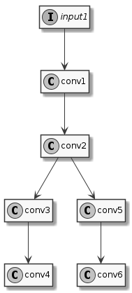
示例模型
This model has one input and six convolutions. We’ve already seen how to compile it with uniform quantization, for example using 16 bits integers:
quantization:
    data_type: int16
Instead of a single type, the data_type field can contain an association map between
layer-names and layer-types. Layer names are those that appear in the model to be converted, it’s
easy to see them using free tools such as Netron. So, the previous example is equivalent to:
quantization:
    data_type:
        input1: int16
        conv1: int16
        conv2: int16
        conv3: int16
        conv4: int16
        conv5: int16
        conv6: int16
To perform mixed-type quantization just select the desired type for each layer. The only limitation
is that uint8 and int8 types can’t be both present at the same time. For example we can
choose to quantize the input and first convolution to 8 bits, the internal convolutions to 16 bits,
and to keep the final convolutions in floating point:
quantization:
    data_type:
        input1: uint8
        conv1: uint8
        conv2: int16
        conv3: int16
        conv4: float16
        conv5: int16
        conv6: float16
Real models can often have well above one hundred layers, so writing an exhaustive list of all the layers
can become confusing and error-prone. To keep the type specification simpler there are a few
shortcuts that can be used. First of all, layers can be omitted: layers not explicitly
listed will be quantized by default to uint8. Furthermore, some special conventions in the layer
name specification can help:
INPUTS : this special name is automatically expanded to the names of all the inputs of the network
‘@layerId’ : a name preceded by the ‘@’ suffix is interpreted as a layerID (see note below)
layername… : a name followed by three dots, is expanded to the names of all the layers that follows the layer specified in the model (in execution order). Useful when for example we want to use the same data type for the head of the network or an entire branch.
'*': expanded to the names of all the layers that haven’t been explicitly specified
The type specifications are applied in the order they are declared (except for ‘*’) so it is possible to further override the type of layers already specified.
备注
During the compilation of a model several optimizations are applied and some layers
in the original network may be fused together or optimized away completely.
For optimized away layers it is of course not possible to specify the data type.
For fused layers the issue is that they will not have the same name as the original layers.
In this case it is possible to identify them by layerId: a layerId is a unique identifier
assigned to each compiled layer. This is also a convenient way to identify layers in case the
original model has layers with ambiguous or empty names. It is possible to see the list of all
layerIDs for a compiled model in the generated quantization_info.yaml
or quantization_entropy.txt file.
Lets’s see a few examples applied to our sample network.
# Quantize input1 as int8, everything else as int16
quantization:
    data_type:
        INPUTS: int8
        '*': int16
# Quantize as uint8 but use int16 for conv3, conv4, conv5, conv6
quantization:
    data_type:
        '*': uint8
        conv2...: int16
# Quantize as uint8 but use int16 for conv3, conv4, conv6 but float16 for conv5
quantization:
    data_type:
        '*': uint8
        conv2...: int16
        conv5: float16
In the two examples above the specification '*': uint8 could have been avoided since uint8
is already the default, but helps in making the intention more explicit.
If we specify the data type for a layer that has been fused, we will get a “Layer name” error at conversion time.
In this case we have to look for the layerId of the corresponding fused layer in quantization_info.yaml
and use the “@” syntax as explained above. For example if in our sample model conv5 and conv6
have been fused, we will get an error if we specify the type for conv5 alone.
Looking in quantization_info.yaml we can find the ID of the fused layer, as in:
'@Conv_Conv_5_200_Conv_Conv_6_185:weight':
We can then use this layer ID in the metafile to specify the data type of the fused layers:
# Quantize as uint8 but use int16 for conv3, conv4, conv6 but float16 for fused conv5+conv6
quantization:
    data_type:
        '*': uint8
        conv2...: int16
        '@Conv_Conv_5_200_Conv_Conv_6_185': float16
异构推理
In some cases it can be useful to execute different parts of a network on different hardware. For example consider an object detection network, where the initial part contains a bunch of convolutions and the final part some postprocessing layer such as TFLite_Detection_PostProcess. The NPU is heavily optimized for executing convolutions, but doesn’t support the postprocessing layer, so the best approach would be to execute the initial part of the network on the NPU and the postprocessing on the CPU.
This can be achieved by specifying the delegate to be used on a per-layer basis, using the same syntax
as we’ve seen for mixed quantization in section 混合量化.
For example, considering again the Model in 示例模型, we can specify that
all layers should be executed on the NPU, except conv5 and the layers that follows it
which we want to execute on the GPU:
# Execute the entire model on the NPU, except conv5 and conv6
delegate:
    '*': npu
    conv5: gpu
    conv5...: gpu
Another advantage of distributing processing to different hardware delegates is that when the model is organized in multiple independent branches (so that a branch can be executed without having to wait for the result of another branch), and each is executed on a different HW unit then the branches can be executed in parallel.
In this way the overall inference time can be reduced to the time it takes to execute the slowest branch. Branch parallelization is always done automatically whenever possible.
备注
Branch parallelization should not be confused with in-layer parallelization, which is also always active when possible. In the example above the two branches (conv3,conv4) and (conv5,conv6) are executed in parallel, the former the NPU and the latter on the GPU. In addition, each convolution layer is parallelized internally by taking advantage of the parallelism available in the NPU and GPU HW.
模型转换教程
Let’s see how to convert and run a typical object-detection model.
Download the sample ssd_mobilenet_v1_1_default_1.tflite object-detection model:
https://tfhub.dev/tensorflow/lite-model/ssd_mobilenet_v1/1/default/1
Create a conversion metafile
ssd_mobilenet.yamlwith the content here below (Important: be careful that newlines and formatting must be respected but they are lost when doing copy-paste from a pdf):outputs: - name: Squeeze dequantize: true format: tflite_detection_boxes y_scale=10 x_scale=10 h_scale=5 w_scale=5 anchors=${ANCHORS} - name: convert_scores dequantize: true format: per_class_confidence class_index_base=-1A few notes on the content of this file:
- “
name: Squeeze” and “name: convert_scores”explicitly specifiy the output tensors where we want model conversion to stop. The last layer (
TFLite_Detection_PostProcess) is a custom layer not suitable for NPU acceleration, so it is implemented in software in theDetectorpostprocessor class.- “
dequantize: true”performs conversion from quantized to float directly in the NPU. This is much faster than doing conversion in software.
- “
tflite_detection_boxes” and “convert_scores”represents the content and data organization in these tensors
- “
y_scale=10” “x_scale=10” “h_scale=5” “w_scale=5”corresponds to the parameters in the
TFLite_Detection_PostProcesslayer in the network- “
${ANCHORS}”is replaced at conversion time with the
anchortensor from theTFLite_Detection_PostProcesslayer. This is needed to be able to compute the bounding boxes during postprocessing.- “
class_index_base=-1”this model has been trained with an additional background class as index 0, so we subtract 1 from the class index during postprocessing to conform to the standard coco dataset labels.
Convert the model (be sure that the model, meta and output dir are in a directory visible in the container, see
-voption in 运行 SyNAP 工具)$ synap convert --model ssd_mobilenet_v1_1_default_1.tflite --meta ssd_mobilenet.yaml --target VS680 --out-dir compiled"Push the model to the board:
$ adb root
$ adb remount
$ adb shell mkdir /data/local/tmp/test
$ adb push compiled/model.synap /data/local/tmp/test
Execute the model:
$ adb shell
# cd /data/local/tmp/test
# synap_cli_od -m model.synap $MODELS/object_detection/coco/sample/sample001_640x480.jpg"

Input image: /vendor/firmware/.../sample/sample001_640x480.jpg (w = 640, h = 480, c = 3)
Detection time: 5.69 ms
#   Score  Class  Position  Size     Description
0   0.70       2  395,103    69, 34  car
1   0.68       2  156, 96    71, 43  car
2   0.64       1  195, 26   287,445  bicycle
3   0.64       2   96,102    18, 16  car
4   0.61       2   76,100    16, 17  car
5   0.53       2  471, 22   167,145  car
模型分析
When developing and optimizing a model it can be useful to understand how the execution time is distributed among the layers of the network. This provides an indication of which layers are executed efficiently and which instead represent bottlenecks.
In order to obtain this information the network has to be executed step by step so that
each single timing can be measured. For this to be possible the network must be generated with
additional profiling instructions by calling synap_convert.py with the --profiling option,
for example:
$ synap convert --model mobilenet_v2_1.0_224_quant.tflite --target VS680 --profiling --out-dir mobilenet_profiling
备注
Even if the execution time of each layer doesn’t change between normal and profiling mode, the overall execution time of a network compiled with profiling enabled will be noticeably higher than that of the same network compiled without profiling, due to the fact that NPU execution has to be started and suspended several times to collect the profiling data. For this reason profiling should normally be disabled, and enabled only when needed for debugging purposes.
备注
When a model is converted using SyNAP toolkit, layers can be fused, replaced with equivalent operations and/or optimized away, hence it is generally not possible to find a one-to-one correspondence between the items in the profiling information and the nodes in the original network. For example adjacent convolution, ReLU and Pooling layer are fused together in a single ConvolutionReluPoolingLayer layer whenever possible. Despite these optimizations the correspondence is normally not too difficult to find. The layers shown in the profiling correspond to those listed in the model_info.txt file generated when the model is converted.
After each execution of a model compiled in profiling mode, the profiling information will be
available in sysfs, see network_profile. Since this information is not persistent
but goes away when the network is destroyed, the easiest way to collect it is by using synap_cli
program. The --profling <filename> option allows to save a copy of the sysfs network_profile file
to a specified file before the network is destroyed:
$ adb push mobilenet_profiling $MODELS/image_classification/imagenet/model/
$ adb shell
# cd $MODELS/image_classification/imagenet/model/mobilenet_profiling
# synap_cli -m model.synap --profiling mobilenet_profiling.txt random

# cat mobilenet_profiling.txt
pid: 21756, nid: 1, inference_count: 78, inference_time: 272430, inference_last: 3108, iobuf_count: 2, iobuf_size: 151529, layers: 34
| lyr |   cycle | time_us | byte_rd | byte_wr | type
|   0 |  152005 |     202 |  151344 |       0 | TensorTranspose
|   1 |  181703 |     460 |    6912 |       0 | ConvolutionReluPoolingLayer2
|   2 |    9319 |      51 |    1392 |       0 | ConvolutionReluPoolingLayer2
|   3 |   17426 |      51 |    1904 |       0 | ConvolutionReluPoolingLayer2
|   4 |   19701 |      51 |    1904 |       0 | ConvolutionReluPoolingLayer2
...
|  28 |   16157 |      52 |    7472 |       0 | ConvolutionReluPoolingLayer2
|  29 |  114557 |     410 |  110480 |       0 | FullyConnectedReluLayer
|  30 |  137091 |     201 |    2864 |    1024 | Softmax2Layer
|  31 |       0 |       0 |       0 |       0 | ConvolutionReluPoolingLayer2
|  32 |       0 |       0 |       0 |       0 | ConvolutionReluPoolingLayer2
|  33 |     670 |      52 |    1008 |       0 | ConvolutionReluPoolingLayer2
与 SyNAP 2.x的兼容
SyNAP 3.x is fully backward compatible with SyNAP 2.x.
It is possible to execute models compiled with SyNAP 3.x toolkit with SyNAP 2.x runtime. The only limitation is that in this case heterogeneous compilation is not available and the entire model will be executed on the NPU. This can be done by specifying the
--out-format nboption when converting the model. In this case the toolkit will generate in output the legacymodel.nbandmodel.jsonfiles instead of themodel.synapfile:$ synap convert --model mobilenet_v2_1.0_224_quant.tflite --target VS680 --out-format nb --out-dir mobilenet_legacyIt is possible to execute models compiled with SyNAP 2.x toolkit with SyNAP 3.x runtime
SyNAP 3.x API is an extension of SyNAP 2.x API, so all the existing applications can be used without any modification
使用 PyTorch 模型
PyTorch framework supports very flexible models where the architecture and behaviour of the network is defined using Python classes instead of fixed graph layers as for example in TFLite.
When saving a model, normally only the state_dict, that is the learnable parameters, are saved and not the model structure itself (
https://pytorch.org/tutorials/beginner/saving_loading_models.html#saving-loading-model-for-inference
).
The original Python code used to define the model is needed to reload the model
and execute it. For this reason there is no way for the toolkit to directly import a PyTorch model
from a .pt file containing only the learnable parameters.
When saving a torch model in a .pt file it is also possible to include references to the Python classes defining the model but even in this case it’s impossible to recreate the model from just the .pt file without the exaact python source tree used to generate it.
A third possibility is to save the model in TorchScript format. In this case the saved model contains both the the learnable parameters and the model structure.
This format can be imported directly using the SyNAP toolkit.
For more info on how to save a model in the TorchScript format see:
An alternative way to save a model in TorchScript format is to use tracing.
Tracing records the operations that are executed when a model is run and is a good way to convert
a model when exporting with torch.jit.script is problematic, for example when the model
has a dynamic structure.
In both cases the generated file will have the same format, so models saved with tracing can also be imported directly.
A detailed comparison of the two techniques is available online searching for “pytorch tracing vs scripting”.
Here below an example of saving a torch model with scripting or tracing:
import torch
import torchvision

# An instance of your model
model = torchvision.models.mobilenet_v2(pretrained=True)

# Switch the model to eval model
model.eval()

# Generate a torch.jit.ScriptModule via scripting
mobilenet_scripted = torch.jit.script(model)

# Save the scripted model in TorchScript format
mobilenet_scripted.save("mobilenet_scripted.torchscript")


# An example input you would normally provide to your model's forward() method.
example = torch.rand(1, 3, 224, 224)

# Generate a torch.jit.ScriptModule via tracing
mobilenet_traced = torch.jit.trace(model, example)

# Save the traced model in TorchScript format
mobilenet_traced.save("mobilenet_traced.torchscript")
重要
Even if there exists multiple possible ways to save a PyTorch model to a file, there is no agreed convention for the extension used in the different cases, and .pt or .pth extension is commonly used no matter the format of the file. Only TorchScript models can be imported with the SyNAP toolkit, if the model is in a different format the import will fail with an error message.
备注
Working with TorchScript models is not very convenient when performing mixed quantization or
heterogeneous inference, as the model layers sometimes don’t have names or the name is modified during the
import process and/or there is not a one-to-one correspondence between the layers in the original
model and the layers in the imported one. The suggestion in this case is to compile the model
with the --preserve option and then look at the intermediate build/model.onnx file
inside the output directory.
An even more portable alternative to exporting a model to TorchScript is to export it to ONNX format. The required code is very similar to the one used to trace the model:
import torch
import torchvision

# An instance of your model
model = torchvision.models.mobilenet_v2(pretrained=True)

# Switch the model to eval model
model.eval()

# Export the model in ONNX format
torch.onnx.export(model, torch.rand(1, 3, 224, 224), "mobilenet.onnx")
导入YOLO PyTorch模型
The popular YOLO library from ultralytics provides pretrained .pt models on their website. All these models are not in TorchScript format and so can’t be imported directly with the SyNAP toolkit. nevertheless it’s very easy to export them to ONNX or TorchScript so that they can be imported:
from ultralytics import YOLO

# Load an official YOLO model
model = YOLO("yolov8s.pt")

# Export the model in TorchScript format
model.export(format="torchscript", imgsz=(480, 640))

# Export the model in ONNX format
model.export(format="onnx", imgsz=(480, 640))
More information on exporting YOLO models to ONNX in https://docs.ultralytics.com/modes/export/
Most publi-domain machine learning packages provide similar export functions for their PyTorch models.